Using eBPF BCC for Non-Intrusive Analysis of Function Execution Time
We all know that monitoring function execution time is crucial when developing and maintaining backend services. Through monitoring, we can promptly identify performance bottlenecks, optimize code, and ensure service stability and response speed. However, traditional methods often involve adding statistics to the code and reporting them, which, although effective, typically only target functions considered to be on the critical path.
Suppose at some point, we suddenly need to monitor the execution time of a function that wasn’t a focus of attention. In this case, modifying the code and redeploying the service can be a cumbersome and time-consuming task. This is where eBPF (extended Berkeley Packet Filter) and BCC (BPF Compiler Collection) come in handy. By using eBPF, we can dynamically insert probes to monitor function execution time without modifying code or redeploying services. This not only greatly simplifies the monitoring process but also reduces the impact on service performance.
In the following article, we will detail how to use eBPF BCC to analyze service function execution time non-intrusively, and demonstrate its powerful capabilities through practical examples.
Principle of eBPF Function Execution Time Analysis
eBPF is a very powerful technology that allows developers to execute custom code in the Linux kernel without modifying the kernel or loading kernel modules. This flexibility makes eBPF applicable to various scenarios, including network monitoring, security, and performance analysis.
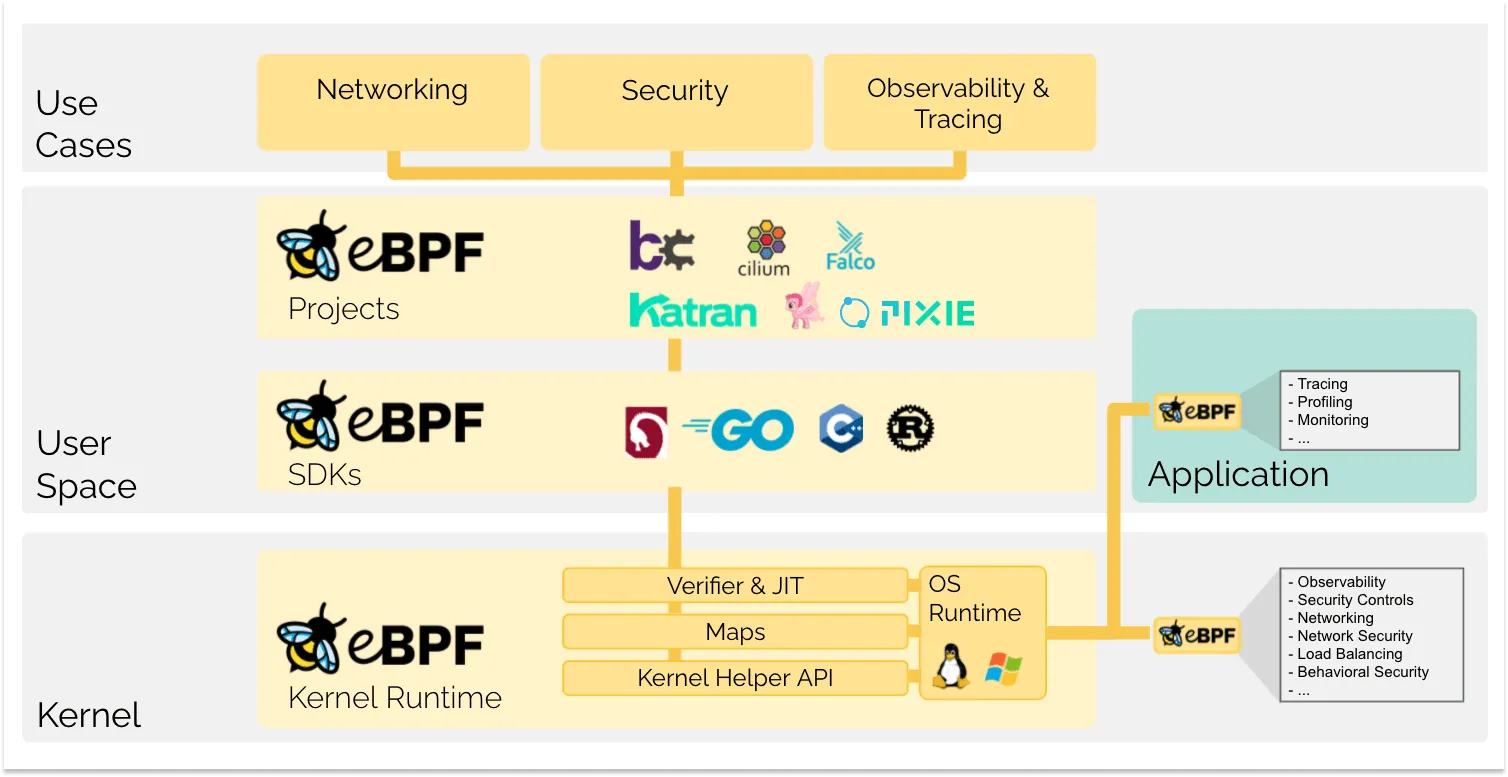
eBPF supports user space tracing (uprobes), allowing us to attach eBPF programs to user space applications. This means we can monitor and analyze the behavior of user space applications very precisely without modifying the application code. We can define code to be executed at function entry and exit points. When a function is called, the entry probe (kprobe/uprobe) is triggered, and when the function returns, the exit probe is triggered.
To calculate the execution time of a function, we can record the current timestamp in the eBPF program at the function entry. In the eBPF program at the function exit, we record the timestamp again and calculate the difference between the two, which is the function’s execution time. The function’s execution time is then stored in BPF Maps for further analysis and visualization in user space, helping us understand the performance characteristics of the function.
Writing eBPF directly can be a bit cumbersome, but fortunately, we can use BCC to simplify the development process. BCC (BPF Compiler Collection) is a development toolkit that simplifies the process of writing and compiling BPF programs, allowing developers to use languages like Python and C to write scripts that control the behavior of eBPF programs.
Simulating Time-Consuming Functions
To use eBPF BCC to analyze function execution time, we first need to create a test process with a specific function that simulates the time consumption of functions in real scenarios. In common business scenarios, the distribution of function execution times is usually uneven, so we’ve intentionally designed a function here to make its P99 latency significantly greater than its average latency. This simulates actual business scenarios where most requests can be processed quickly, but in some cases (such as large data volumes, cache misses, or resource contention), processing time increases significantly.
To add a bit more explanation, P99 latency is a performance metric that describes the 99th percentile of execution times in a system or function. You can understand it simply like this: if you have 100 requests, the P99 latency is the execution time of the slowest one among these 100 requests. However, different tools may calculate P99 slightly differently. For example, if a function is executed 100 times, with 99 executions taking between 1ms and 2ms, and one execution taking 100ms, the P99 could be either 2ms or 100ms, depending on the specific algorithm implementation. This doesn’t affect our understanding of the P99 metric here.
Here’s the implementation of our simulated time-consuming function:
1 | void someFunction(int iteration) { |
To provide a baseline for time consumption, we’ve also added time statistics in our test code to calculate the function’s average and P99 latency. Specifically, in an infinite loop, it calls the function each time and records the execution time. Whenever the cumulative execution time exceeds one second, it calculates and outputs the average and P99 times of the function executions during this period. Then, it clears all recorded execution times, ready to start the next round of data collection and analysis. Here’s the implementation:
1 | int main() { |
The complete code func_time.cpp is available on gist. On my server, the execution results are as follows (note that function execution time is related to machine performance and load):
Average execution time: 3.95762 ms
P99 execution time: 190.968 ms
Average execution time: 3.90211 ms
P99 execution time: 191.292 ms
…
BCC Function Execution Time Histogram
Note that the latency monitoring script here depends on the BCC tool. You can find installation instructions on BCC’s GitHub page. Additionally, ensure that your system kernel supports BPF. For Linux kernel versions, typically 4.8 or above is needed for the best BPF functionality support.
BCC provides convenient methods for us to statistics the distribution of function execution times. First, it obtains the target process PID and the function name to be traced by parsing command line arguments. Then it builds and loads a BPF program, attaching user-space probes (uprobes) and user-space return probes (uretprobes) to the specified process and function to capture timestamps at the beginning and end of the function.
The probe function trace_start captures the current timestamp each time a function call begins, and stores it in the BPF hash map start along with a key representing the current process. When the function call ends, the trace_end probe function looks up the start timestamp and calculates the time difference of the function execution. This time difference is recorded in the BPF histogram dist for subsequent performance analysis. The complete script func_time_hist.py is available on gist.
1 | int trace_start(struct pt_regs *ctx) { |
We compile func_time.cpp with -g, and use nm to get the name-mangled function name. Run the program, get the process pid, and then we can use the tool to view the execution time distribution.
1 | g++ func_time.cpp -g -o func_time |
When you press Ctrl-C to abort the program, it will print out the dist histogram, showing the distribution of function execution times on a logarithmic scale. This allows us to quickly understand the general performance of function execution, such as the most common execution time and the range of time distribution, as shown in the following figure:
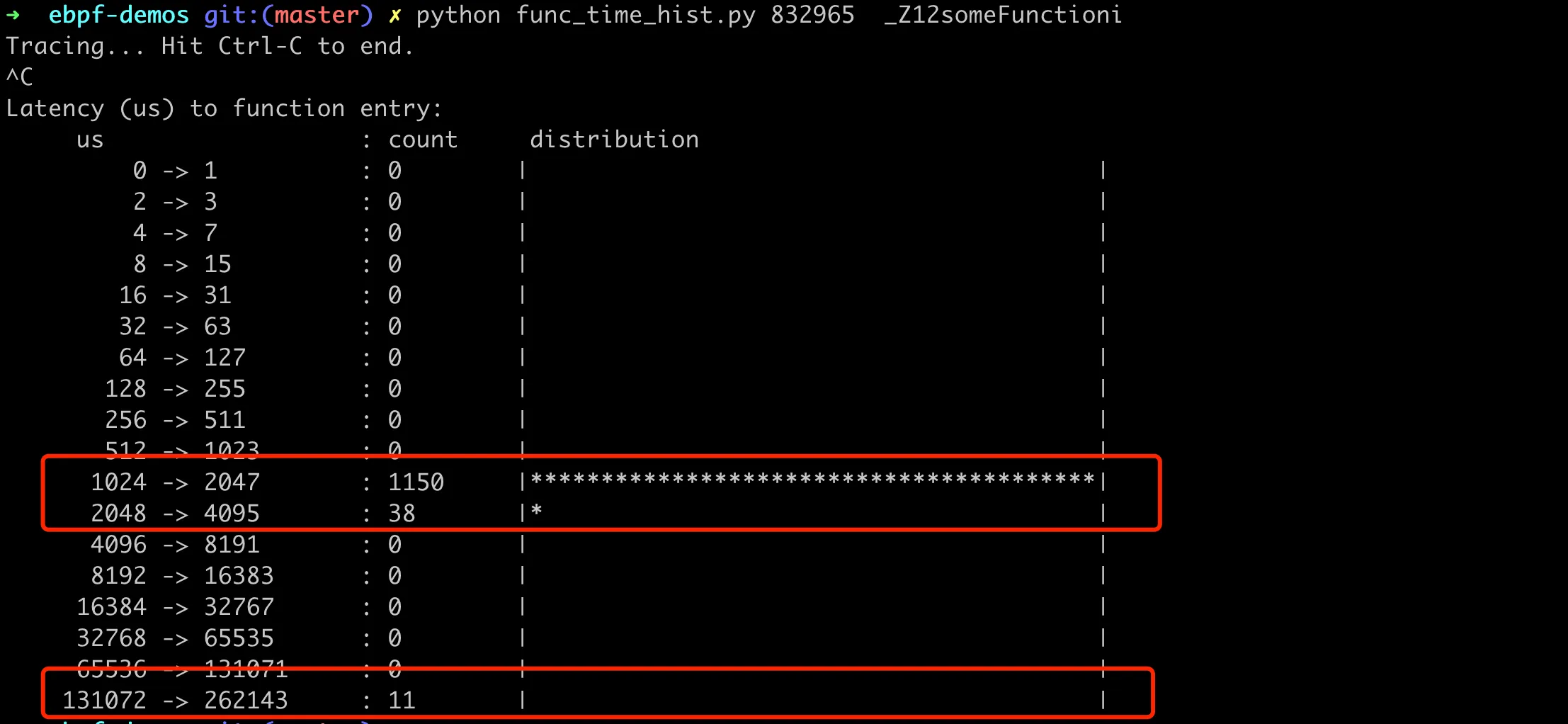
We can see that most function calls have execution times distributed between 1024-2047us, with 11 function calls having execution times distributed between 131702-262143us. This function proportion is about 1%, which matches the characteristics of our simulated function.
BCC Function Average Execution Time
Often, we not only want to see the distribution of function execution times but also want to know the average and P99 latency. This can be achieved by making slight modifications to the above BCC script. After each function execution, use BPF’s PERF output interface to collect execution times to user space. Specifically, this is implemented by using the perf_submit helper function in the trace_end function of the BPF program.
1 | int trace_end(struct pt_regs *ctx) { |
Next, in the Python script in user space, calculate the average and P99 within each specified time interval. The complete code func_time.py is available on gist, with execution results as follows:
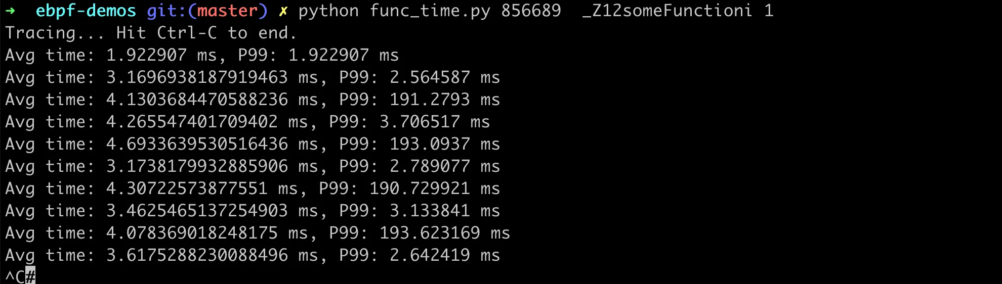
Overall, using eBPF and BCC for this kind of non-intrusive performance analysis has enormous value for troubleshooting and performance optimization in production environments. It allows us to collect and analyze critical performance metrics in real-time without interrupting services or redeploying code. This capability is crucial for maintaining high-performance and high-availability systems.

