LevelDB Explained - Bloom Filter Implementation and Visualization

In LevelDB, data is stored in SSTable files. When using Get() to query a key, it may be necessary to read multiple blocks from the SST file. To reduce disk reads, LevelDB provides a FilterPolicy strategy. If it can determine that a key is not in the current SSTable file, it can skip reading that file, thus improving query efficiency.

LevelDB supports user-defined filter policies but provides a default Bloom filter implementation. A Bloom filter is a space-efficient data structure used to determine whether an element is a member of a set. It has a certain false positive rate but no false negatives. In simple terms, if a Bloom filter determines that an element does not exist, then the element definitely does not exist; if a Bloom filter determines that an element exists, then the element may not exist.

Using a Bloom filter in LevelDB is quite simple, as shown in the following code:

leveldb::Options options;
options.filter_policy = NewBloomFilterPolicy(10);
leveldb::DB* db;
leveldb::DB::Open(options, "/tmp/testdb", &db);
// ... use the database ...
delete db;
delete options.filter_policy;

So what are the principles behind Bloom filters? And how are they implemented in LevelDB? Let’s take a look together in this article.

LevelDB Interface Definition

Before delving into the implementation details of Bloom filters, let’s first look at how LevelDB defines the filter interface.

LevelDB defines the interface for filter policies in filter_policy.h. FilterPolicy itself is an abstract class that defines 3 pure virtual functions as interfaces. It cannot be instantiated directly and must be implemented by subclasses.

class LEVELDB_EXPORT FilterPolicy {
 public:
  virtual ~FilterPolicy();

  virtual const char* Name() const = 0;

  virtual void CreateFilter(const Slice* keys, int n,
                            std::string* dst) const = 0;

  virtual bool KeyMayMatch(const Slice& key, const Slice& filter) const = 0;
};

All three of these interfaces are important, and the code comments explain them in detail:

• Name(): Returns the name of the filter policy, which is very important for version compatibility. If the implementation of the filter policy (i.e., data structure or algorithm) changes, potentially causing incompatibility with old versions, the returned name should reflect this change to prevent old filter policies from being used incorrectly.
• CreateFilter(): Used to create a filter, i.e., adding all keys in keys to the filter and then saving the content in dst.
• KeyMayMatch(): Used to determine if a key exists in the filter, where filter is the dst generated by CreateFilter(). If the key exists in the filter, it must return true. If it doesn’t exist, it can return either true or false, but the probability of returning false should be as high as possible.

Additionally, a factory function is provided to create a Bloom filter instance. However, one drawback is that after using the returned filter policy instance, you need to remember to manually release the resources. The use of a factory function here allows library maintainers to change the object creation process without affecting existing client code. For example, if a more efficient Bloom filter implementation is developed in the future, the factory function can simply be modified to return the new implementation without needing to modify the code that calls it. This provides convenience for future expansion and maintenance.

LEVELDB_EXPORT const FilterPolicy* NewBloomFilterPolicy(int bits_per_key);

By defining the filter policy interface and using a factory function, developers can easily implement different filter policies. To implement a new filter policy, you only need to inherit the FilterPolicy class and implement the corresponding methods. For the caller, they only need to pass the new filter policy to the Options object, and the overall changes will be relatively simple.

Bloom Filter Principles

LevelDB implemented its own Bloom filter as the default filter policy. Before we start looking at the implementation code, let’s first understand the principles of Bloom filters.

In 1970, Burton Howard Bloom created the Bloom filter, an efficient data structure, to check whether an English word is in the dictionary for a spell checker. Its core is an m-bit bit array and k hash functions. The core operations are as follows:

1. Initialization: At the start, the Bloom filter is an array of m bits, with each bit set to 0.
2. Adding elements: When adding an element to the Bloom filter, first use k hash functions to hash the element, producing k array position indices, then set all these positions to 1.
3. Querying elements: To check if an element is in the Bloom filter, use the same k hash functions to hash the element, obtaining k indices. If all these indices correspond to bits that are 1, then the element may exist in the set; if any bit is 0, then the element definitely does not exist in the set.

From the above description, we can see that the time required to add or check whether an element is in the set is a fixed constant $O\left(k\right)$, completely independent of the number of elements already in the set. Compared to other data structures representing sets, such as hash tables, balanced binary trees, skip lists, etc., in addition to fast lookup speed, Bloom filters are also very space-efficient as they don’t need to store the elements themselves, saving considerable space.

However, Bloom filters also have drawbacks. Careful consideration of the above process reveals that the query results of Bloom filters can be false positives. Bloom filters use multiple hash functions to process each element, setting multiple resulting positions to 1, and these positions may overlap with the hash results of other elements. Suppose a key does not exist in the set, but its hash results overlap with the hash results of other elements. In this case, the Bloom filter would determine that this key exists in the set, which is known as a false positive.

The probability that a Bloom filter incorrectly determines an element exists when it actually does not is called the false positive rate. Intuitively, for a fixed number k of hash functions, the larger the array size m, the fewer hash collisions, and thus the lower the false positive rate. To design a good Bloom filter ensuring a very low false positive rate, this qualitative analysis is not enough; we need to perform mathematical derivation for quantitative analysis.

Mathematical Derivation

Here’s a simple derivation of the Bloom filter error rate calculation. You can skip this part and directly read the LevelDB Implementation section. Assume the bit array size of the Bloom filter is $\left(m\right)$, the number of hash functions is $\left(k\right)$, and $\left(n\right)$ elements have been added to the filter. We assume that the hash functions we use are very random, so we can assume that the hash functions choose positions in the array with equal probability. During the insertion of elements, the probability of a certain bit being set to 1 by a certain hash function is $\left(\frac{1}{m}\right)$, and the probability of not being set to 1 is $(1-\frac{1}{m})$.

$k$ is the number of hash functions, and the hash functions we choose are uncorrelated and independent of each other. So the probability of a bit not being set to 1 by any hash function is:

$${\left(1-\frac{1}{m}\right)}^k$$

Next is a mathematical trick. The natural logarithm $e$ has an identity:

$$\underset{m\to \infty }{lim}{\left(1-\frac{1}{m}\right)}^m=\frac{1}{e}$$

For relatively large m, we can deduce:

$${\left(1-\frac{1}{m}\right)}^k={\left({\left(1-\frac{1}{m}\right)}^m\right)}^{k/m}\approx e^{-k/m}$$

We have inserted n elements, so the probability of a certain bit not being set to 1 is:

$${\left(1-\frac{1}{m}\right)}^{kn}\approx e^{-kn/m}$$

Therefore, the probability of a certain bit being set to 1 is:

$$1-{\left(1-\frac{1}{m}\right)}^{kn}\approx 1-e^{-kn/m}$$

Assuming an element is not in the set, the probability that all k bits are set to 1 is:

$${\left(1-e^{-kn/m}\right)}^k$$

Parameter Selection

From the above derivation, we can see that the false positive rate is related to the number of hash functions $k$, the size of the bit array $m$, and the number of added elements $n$.

• $n$ is usually determined by the application scenario, representing the expected total number of elements to be inserted into the Bloom filter. It can be predicted, determined by external factors, and is not easily adjustable.
• Increasing $m$ can directly reduce the false positive rate, but this will increase the storage space requirements of the Bloom filter. In storage-constrained environments, you may not want to increase it indefinitely. Additionally, the effect of expanding $m$ is linear, and you need to balance performance improvement with additional storage costs.
• Changing $k$ has a very significant impact on the false positive rate because it directly affects the probability of bits in the bit array being set to 1.

Considering all these factors, in practical applications, $n$ is determined by the usage scenario, while $m$ is limited by storage costs, making adjusting $k$ a practical and direct optimization method. Given the expected number of elements $n$ and the bit array size $m$, we need to find an appropriate k that minimizes the false positive rate.

Finding the appropriate k here is an optimization problem that can be solved mathematically. It’s quite complex, so we’ll just state the conclusion. The optimal $\left(k\right)$ is as follows:

$$k=\frac{m}{n}\ln 2$$

LevelDB Implementation

Above, we introduced the principles of Bloom filters. Now let’s see how they are specifically implemented in LevelDB. The implementation of Bloom filters in LevelDB is in bloom.cc, where BloomFilterPolicy inherits from FilterPolicy and implements the aforementioned interfaces.

Hash Function Count Selection

First, let’s look at the selection of the number of hash functions k. The code is as follows:

explicit BloomFilterPolicy(int bits_per_key) : bits_per_key_(bits_per_key) {
  // We intentionally round down to reduce probing cost a little bit
  k_ = static_cast<size_t>(bits_per_key * 0.69);  // 0.69 =~ ln(2)
  if (k_ < 1) k_ = 1;
  if (k_ > 30) k_ = 30;
}

The bits_per_key parameter is passed in when constructing the Bloom filter, and LevelDB always passes 10. This value represents the average number of bits occupied by each key, i.e., $\frac{m}{n}$. The 0.69 here is an approximation of $\ln \left(2\right)$, and this coefficient comes from the optimal hash function count formula $k=\frac{m}{n}\ln 2$ discussed above. Finally, some boundary protection is performed here to ensure that the value of k is between 1 and 30, avoiding k being too large and making hash calculations too time-consuming.

Creating the Filter

Next, let’s see how the filter is created here. The complete code is as follows:

void CreateFilter(const Slice* keys, int n, std::string* dst) const override {
  // Compute bloom filter size (in both bits and bytes)
  size_t bits = n * bits_per_key_;

  // For small n, we can see a very high false positive rate.  Fix it
  // by enforcing a minimum bloom filter length.
  if (bits < 64) bits = 64;

  size_t bytes = (bits + 7) / 8;
  bits = bytes * 8;

  const size_t init_size = dst->size();
  dst->resize(init_size + bytes, 0);
  dst->push_back(static_cast<char>(k_));  // Remember # of probes in filter
  char* array = &(*dst)[init_size];
  for (int i = 0; i < n; i++) {
    // Use double-hashing to generate a sequence of hash values.
    // See analysis in [Kirsch,Mitzenmacher 2006].
    uint32_t h = BloomHash(keys[i]);
    const uint32_t delta = (h >> 17) | (h << 15);  // Rotate right 17 bits
    for (size_t j = 0; j < k_; j++) {
      const uint32_t bitpos = h % bits;
      array[bitpos / 8] |= (1 << (bitpos % 8));
      h += delta;
    }
  }
}

First, it calculates the space needed for the bit array, based on the number of keys $n$ and the average number of bits per key. It also considers some boundary conditions: if the resulting number of bits is too small (less than 64 bits), it sets it to 64 bits to avoid a high false positive rate. Additionally, it considers byte alignment, converting the number of bits to bytes while ensuring the total number of bits is a multiple of 8.

Next, it uses resize to increase the size of dst, allocating space for the bit array after the target string. Here, the Bloom filter is designed to be appended to existing data without overwriting or deleting existing data. The newly added space is initialized to 0 because the Bloom filter’s bit array needs to start from an all-zero state. Then k_, the number of hash functions, is added to the end of the target string dst. This value is part of the Bloom filter’s metadata and is used to determine how many hash calculations need to be performed when querying whether a key exists.

Finally, there’s the core part of the Bloom filter, calculating which bit array positions need to be set to 1. Normally, you would need to set up k hash functions, calculate k times, and then set the corresponding positions. However, LevelDB’s implementation seems different. For each key, it uses the BloomHash function to calculate the initial hash value h of the key, then sets the corresponding position. In subsequent calculations, each time it right-shifts the previous hash value by 17 bits, left-shifts by 15 bits, and then performs an OR operation to calculate delta. Then it adds delta to the previous hash value to calculate the next hash value. This way, it can obtain k hash values and then set the corresponding positions.

In the previous Mathematical Derivation section, we mentioned that these k hash functions need to be random and mutually independent. Can the above method meet this requirement? The code comment mentions that it adopts the double-hashing method, referring to the analysis in [Kirsch,Mitzenmacher 2006]. Although the hash values generated by double hashing are not as completely unrelated as those from completely independent hash functions, in practical applications, they provide sufficient randomness and independence to meet the requirements of Bloom filters.

The advantages here are also obvious. Double hashing can generate multiple pseudo-independent hash values from one basic hash function, without needing to implement k hashes, making the implementation very simple. Moreover, compared to multiple independent hash functions, the double hashing method reduces computational overhead because it only needs to calculate one real hash value, with the rest of the hash values obtained through simple arithmetic and bit operations.

Querying Key Existence

Finally, let’s look at how to query whether a key exists. If you understood the previous part about creating the filter, this part should be easy to understand. The complete code is as follows:

bool KeyMayMatch(const Slice& key, const Slice& bloom_filter) const override {
  const size_t len = bloom_filter.size();
  if (len < 2) return false;

  const char* array = bloom_filter.data();
  const size_t bits = (len - 1) * 8;

  // Use the encoded k so that we can read filters generated by
  // bloom filters created using different parameters.
  const size_t k = array[len - 1];
  if (k > 30) {
    // Reserved for potentially new encodings for short bloom filters.
    // Consider it a match.
    return true;
  }

  uint32_t h = BloomHash(key);
  const uint32_t delta = (h >> 17) | (h << 15);  // Rotate right 17 bits
  for (size_t j = 0; j < k; j++) {
    const uint32_t bitpos = h % bits;
    if ((array[bitpos / 8] & (1 << (bitpos % 8))) == 0) return false;
    h += delta;
  }
  return true;
}

The beginning part is just some boundary condition checks. If the filter length is less than 2, it returns false. It reads the value of k from the last byte of the filter data, which was stored when creating the filter and is used to determine how many hash calculations need to be performed. If k is greater than 30, this case is considered as possibly for future new encoding schemes, so the function directly returns true, assuming the key might exist in the set (as of 2024, no new encoding schemes have been extended here).

The next part is similar to when creating the filter. It uses the BloomHash function to calculate the hash value of the key, then performs bit rotation to generate delta, which is used to modify the hash value in the loop to simulate the effect of multiple hash functions. During this process, if any bit is 0, it indicates that the key is definitely not in the set, and the function returns false. If all relevant bits are 1, it returns true, indicating that the key might be in the set.

Bloom Filter Testing

The implementation of Bloom filters in LevelDB also provides complete test code, which can be found in bloom_test.cc.

First, the BloomTest class is derived from the testing::Test class, used to organize and execute test cases related to Bloom filters. Its constructor and destructor are used to create and release instances of NewBloomFilterPolicy, ensuring that each test case can run in a clean environment. The Add method is used to add keys to the Bloom filter, and Build converts the collected keys into a filter. The Matches method is used to check whether a specific key matches the filter, while the FalsePositiveRate method is used to evaluate the false positive rate of the filter.

Then there’s a series of specific test cases defined by the TEST_F macro, allowing each test case to automatically possess the methods and properties defined in the BloomTest class. The first two test cases are relatively simple:

• EmptyFilter: Tests an empty filter, i.e., whether the filter can correctly determine that a key does not exist when no keys have been added.
• Small: Tests the case of adding a small number of keys, checking whether the filter can correctly determine if keys exist.

It’s worth noting the VaryingLengths test case, which is a more complex test case used to evaluate and verify the performance and efficiency of the Bloom filter under different data scales (i.e., different numbers of keys). By using the defined NextLength function to incrementally increase the number of keys, it tests the performance of the Bloom filter under different key set sizes. It mainly tests the following three aspects:

1. Ensures that the size of the constructed Bloom filter is within the expected range;
2. Ensures that all keys added to the filter can be correctly identified as existing;
3. Evaluates the false positive rate (false positive rate) of the Bloom filter at different lengths, ensuring that the false positive rate does not exceed 2%. At the same time, it categorizes filters as “good” or “mediocre” based on their false positive rates, and performs statistics and comparisons on their numbers, ensuring that the number of “mediocre” filters is not too high.

The complete test code is as follows:

  TEST_F(BloomTest, VaryingLengths) {
  char buffer[sizeof(int)];

  // Count number of filters that significantly exceed the false positive rate
  int mediocre_filters = 0;
  int good_filters = 0;

  for (int length = 1; length <= 10000; length = NextLength(length)) {
    Reset();
    for (int i = 0; i < length; i++) {
      Add(Key(i, buffer));
    }
    Build();

    ASSERT_LE(FilterSize(), static_cast<size_t>((length * 10 / 8) + 40))
        << length;

    // All added keys must match
    for (int i = 0; i < length; i++) {
      ASSERT_TRUE(Matches(Key(i, buffer)))
          << "Length " << length << "; key " << i;
    }

    // Check false positive rate
    double rate = FalsePositiveRate();
    if (kVerbose >= 1) {
      std::fprintf(stderr,
                   "False positives: %5.2f%% @ length = %6d ; bytes = %6d\n",
                   rate * 100.0, length, static_cast<int>(FilterSize()));
    }
    ASSERT_LE(rate, 0.02);  // Must not be over 2%
    if (rate > 0.0125)
      mediocre_filters++;  // Allowed, but not too often
    else
      good_filters++;
  }
  if (kVerbose >= 1) {
    std::fprintf(stderr, "Filters: %d good, %d mediocre\n", good_filters,
                 mediocre_filters);
  }
  ASSERT_LE(mediocre_filters, good_filters / 5);
}

Here’s the result of executing the test:

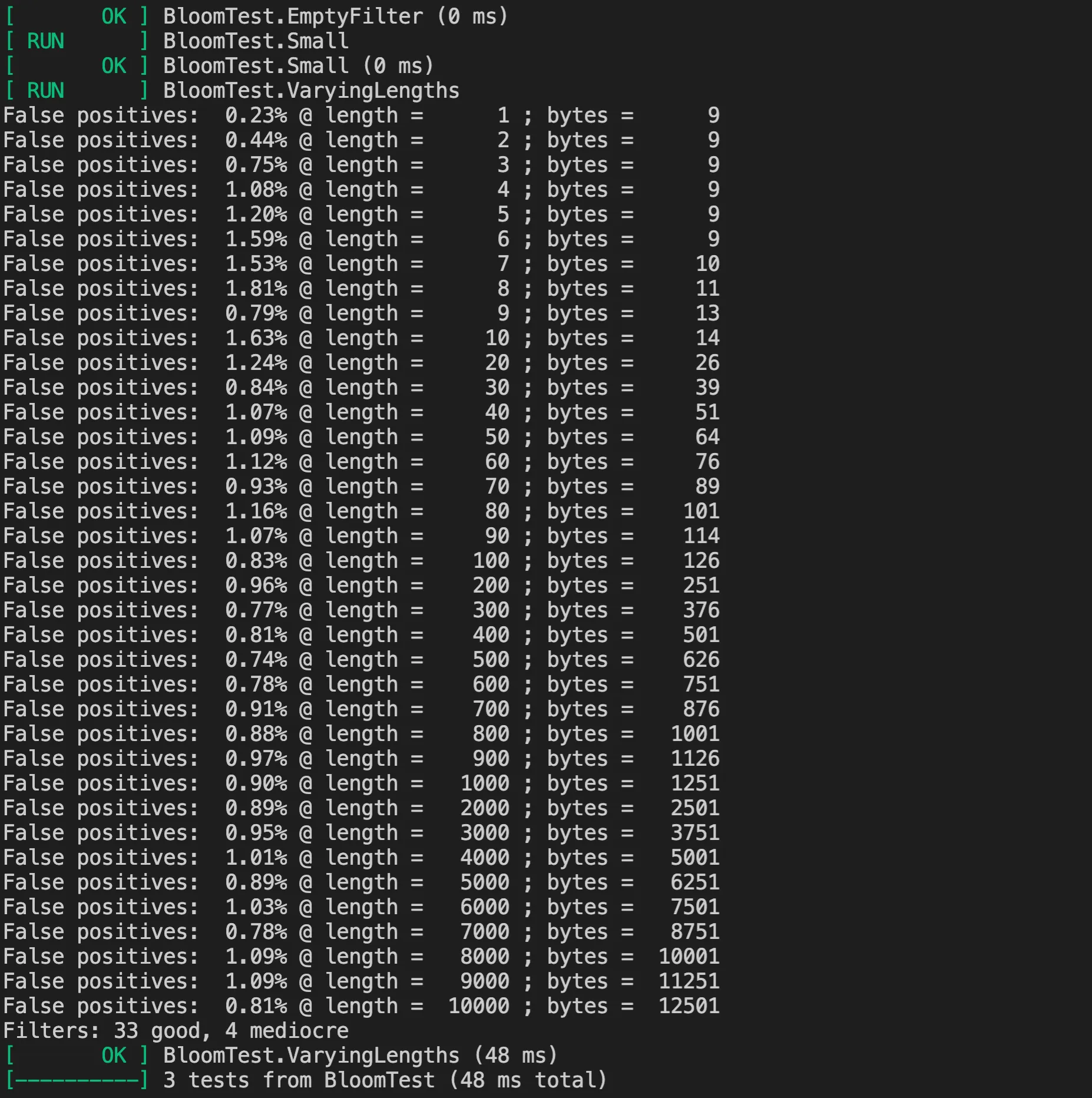Bloom Filter Test Results

Bloom Filter Visualization

Before concluding the article, let’s take a look at a visualization demonstration of the Bloom filter, which displays the principles and implementation discussed above in the form of charts, deepening our understanding.

Bloom Filter Visualization Demo

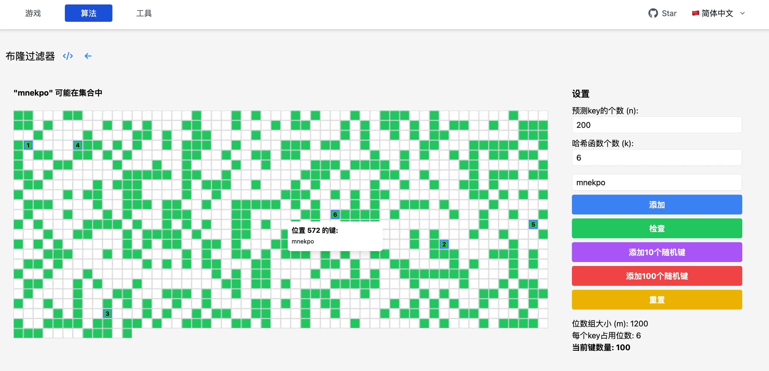
In this demonstration site, you can choose different numbers of hash functions and predicted key counts. It will then automatically adjust the bit array. After that, you can add elements and check if elements are in the Bloom filter. If an element is present, the corresponding array bits will be displayed with black boxes. If it’s not present, the corresponding array bits will be displayed with red boxes. This allows for an intuitive understanding of how Bloom filters work.

Also, for ease of demonstration, clicking on a bit group will show which keys would hash to this location. In reality, Bloom filters don’t store this information; it’s stored additionally here just for demonstration purposes.

Summary

Bloom filters are an efficient data structure used to determine whether an element exists in a set. Its core is a bit array and multiple hash functions, using multiple hash calculations to set bits in the bit array. Through rigorous mathematical derivation, we can conclude that the false positive rate of Bloom filters is related to the number of hash functions, the size of the bit array, and the number of added elements. In practical applications, the false positive rate can be optimized by adjusting the number of hash functions.

LevelDB implemented a Bloom filter as the default filter policy, which can be created through a factory function, maintaining extensibility. To save hash resource consumption, LevelDB generates multiple pseudo-independent hash values through the double hashing method, then sets the corresponding bits. When querying, it also uses multiple hash calculations to determine whether a key exists in the set. LevelDB provides complete test cases to verify the correctness and false positive rate of the Bloom filter.

Additionally, to intuitively understand how Bloom filters work, I’ve created a visualization demonstration of Bloom filters here, showing the principles of Bloom filters through charts.