LevelDB Explained - How to Analyze the Time Complexity of SkipLists?
In the previous article LevelDB Explained - How to implement SkipList, we analyzed in detail the implementation of skip lists in LevelDB. Then in LevelDB Explained - How to Test Parallel Read and Write of SkipLists?, we analyzed the test code for LevelDB skip lists. One question remains: how do we analyze the time complexity of skip lists?
After analyzing the time complexity of skip lists, we can understand the choice of probability value and maximum height in LevelDB, as well as why Redis chooses a different maximum height. Finally, this article will also provide a simple benchmark code to examine the performance of skip lists.
This article will not involve very advanced mathematical knowledge, only simple probability theory, so you can read on without worry. The performance analysis of skip lists has several approaches worth learning from. I hope this article can serve as a starting point and bring some inspiration to everyone.
Breaking Down Skip List Performance Analysis
Knowing the principles and implementation of LevelDB, we can deduce that in extreme cases, where the height of each node is 1, the time complexity of search, insertion, and deletion operations of the skip list will degrade to O(n). In this case, the performance is considerably worse than balanced trees. Of course, due to the randomness involved, no input sequence can consistently lead to the worst performance.
So, how about the average performance of skip lists? We’ve previously stated the conclusion that it’s similar to the average performance of balanced trees. Introducing a simple random height can ensure that the average performance of skip lists is comparable to balanced trees. Is there any analysis method behind this that can analyze the performance of skip lists?
We need to look at the paper again. The paper provides a good analysis method, but the approach here is actually a bit difficult to come up with, and understanding it is also a bit challenging. I will try to break down the problem as much as possible, then derive the entire process step by step, and try to provide the mathematical derivation involved in each step. Haha, isn’t this the chain of thought? Breaking down problems and reasoning step by step is an essential skill for both humans and AI to solve complex problems. The derivation here can be divided into several small problems:
- Among the search, insertion, and deletion operations of skip lists, which part of the operation most affects the time consumption?
- For the search operation, assuming we start searching downwards from any level k, what is the average complexity here (how many traversals)?
- Is there a way to find a certain level in the linked list, from which starting the search is most efficient, and the number of traversals can represent the average performance?
- Can we find a formula to calculate the total time complexity and calculate the upper limit of the average complexity here?
Alright, let’s analyze these problems one by one.
Bottleneck of Skip List Operations
The first small problem is relatively simple. In the previous discussion of the principles and implementation of skip lists, we know that for insertion and deletion operations, we also need to first find the corresponding position through the search operation. After that, it’s just a few pointer operations, the cost of which is constant time and can be ignored. Therefore, the time complexity of skip list operations is determined by the complexity of the search operation.
The process of the search operation is to search right and down in the skip list until the target element is found. If we can know the average complexity of this search, then we can know the average complexity of skip list operations. Directly analyzing the average complexity of the search operation is a bit difficult to start. According to the implementation in LevelDB, each time it starts searching from the highest level of the current node in the skip list. But the node height is random, and the highest level is also random, so it seems impossible to analyze the average complexity of the search operation starting from a random height.
Expected Number of Steps to Skip k Levels
Let’s give up on direct analysis for now and try to answer the second question from earlier. Assuming we start searching downwards from any level k, how many times on average does it take to find the target position? The analysis approach here is quite jumpy. We’ll analyze in reverse from the target position, searching up and left, how many steps on average does it take to search up k levels. And we assume that the height of nodes in the linked list is randomly decided based on probability p during the reverse search process.
Is this assumption and analysis process equivalent to the average number of searches in the real search situation? We know that when executing the search to the right and down, the heights of the nodes are already decided. But considering that the height of nodes is randomly decided in the first place, assuming that the height is decided during the reverse search and reversing the entire search process is not statistically different.
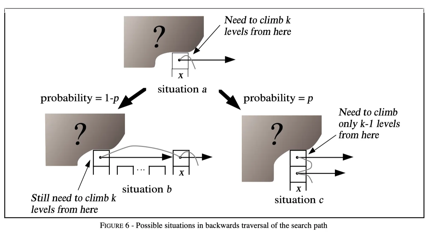
Next, let’s assume that we are currently at any level i of node x (situation a in the figure below), and it takes $ C(k) $ steps to search up k levels from this position. We don’t know if there are any more levels above node x, nor do we know if there are any nodes to the left of node x (the shaded question marks in the figure below represent this uncertainty). Let’s further assume that x is not the header node, and there are nodes to its left (in fact, for this analysis, we can assume there are infinitely many nodes to the left).

Then there are two possible situations for the entire linked list, as shown in the figure above:
- Situation b: Node x has a total of i levels, there are nodes to the left, and when searching, we need to horizontally jump from the i-th level of the left node to the i-th level of x. In reverse analysis, because we decide whether to have a higher level based on probability $ p $, the probability of being in situation b is $ 1 - p $. Then the left node and x are on the same level, and it still takes $ C(k) $ steps to search up k levels. Therefore, the expected number of search steps in this situation is: $ (1 - p) * (C(k) + 1) $.
- Situation c: The height of node x is greater than i, so when searching, we need to jump down from the i+1-th level of x to the i-th level. In reverse analysis, because we decide whether to have a higher level based on probability $ p $, the probability of being in situation c is $ p $. Then searching up k levels from the i+1-th level is equivalent to searching up k-1 levels from the i-th level, which takes $ C(k-1) $ steps. Therefore, the expected number of search steps is: $ p * (C(k-1) + 1) $.
That is to say, for searching starting from any level i, the expected number of steps to jump up $ k $ levels is:
$$ \begin{align}
C(k) &= (1 - p) * (C(k) + 1) + p * (C(k-1) + 1)
\end{align} $$
Simplifying this equation gives the following result:
$$
\begin{align}
C(k) &= 1/p + C(k-1)
\\
C(k) &= k/p
\end{align}
$$
The expected number of steps $ k/p $ to jump up k levels starting from any level i here is also equivalent to the expected number of steps needed to search from level k to the target position at the bottom level in the normal search procedure. This formula is very important. As long as you understand the reverse analysis steps here, the final formula is also relatively easy to derive. However, we still can’t directly analyze the average performance of skip lists with this formula. Something is missing in between.
From Which Level to Start Searching?
From the above analysis, we can see that the time complexity of searching from the K-th level to the bottom level is $ k/p $. So when actually searching the skip list, which level is better to start searching from? From LevelDB Source Code Reading: Principles, Implementation, and Visualization of Skip Lists, we know that the level height of nodes in the skip list is random, for a certain level, there may be multiple nodes, and the higher the level, the fewer the nodes.
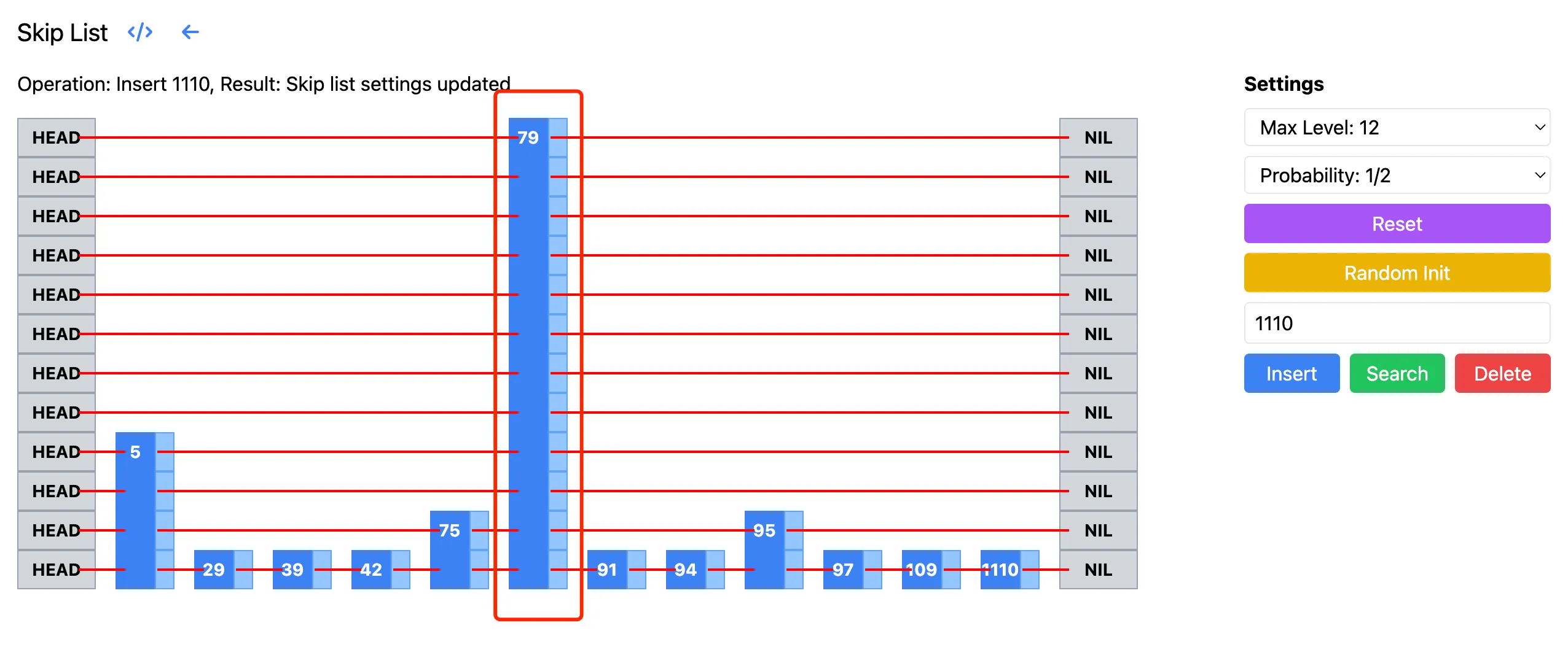
In LevelDB’s implementation, it starts searching from the highest level of the skip list. But in fact, if you start searching from the highest level, you might be doing a lot of unnecessary work. For example, in the skip list below, the level corresponding to 79 is very high. Starting the search from this level requires going down many steps, which are all ineffective searches. If we start searching from the level height corresponding to 5, we save a lot of search steps. The following image is from the skip list visualization page:

Ideally, we want to start searching from an “appropriate“ level. The paper defines the appropriate level as: the level where we expect to see $1/p$ nodes. Since we usually choose values like 1/2, 1/4 for p, we generally start searching from a level with 2 or 4 nodes. Starting the search from this level avoids doing unnecessary work and also avoids losing the advantages of skip lists by starting from too low a level. Next, we only need to know how high such a level is on average, and then combine it with the previous $ k/p $ to know the overall search complexity.
Level Height Calculation
Now let’s look at the specific calculation steps. Assume there are $ n $ nodes in total, and there are $ 1/p $ nodes at the $ L $-th level. Since we decide whether to jump to the upper level with probability $ p $ each time, we have:
$$ n * p^{L-1} = 1/p $$
Note that jumping L levels means jumping L-1 times, so $ p^{L-1} $ here is to the power of L-1. Multiplying both sides of the equation by p:
$$
\begin{align}
(n \cdot p^{L-1}) \cdot p &= \frac{1}{p} \cdot p \\
n \cdot p^{L} &= 1
\end{align}
$$
Then take the logarithm $ log_{1/p} $ on both sides, as follows. Here we use the multiplication rule and power rule of logarithms:
$$
\begin{align}
\log_{1/p} (n \cdot p^{L}) &= \log_{1/p} 1
\\
\log_{1/p} n + L \cdot \log_{1/p} p &= 0
\end{align}
$$
Then simplify:
$$
\begin{align}
log_{1/p} p &= -1
\\
log_{1/p} n + L * (-1) &= 0
\end{align}
$$
So we get:
$$
L = log_{1/p} n
$$
That is, at level $ L = log_{1/p} n$, we expect to have $ 1/p $ nodes. Here’s a supplement to the logarithm rules used in the above derivation:
$$
\begin{align}
\log(xy) &= \log(x) + \log(y) &\text{Multiplication rule of logarithms}
\\
\log(x^n) &= n \cdot \log(x) &\text{Power rule of logarithms}
\end{align}
$$
Total Time Complexity
Alright, the key parts have been analyzed. Now let’s look at the total time complexity by combining the above conclusions. For a skip list with $n$ nodes, we can divide the search process into two parts: one is from the $L$-th level to the bottom level, and the other is from the top to the $L$-th level.
From the $L$-th level to the bottom level, according to the equivalent reverse analysis earlier, it’s equivalent to climbing up $L$ levels from the bottom level. The cost of this climb is:
$$
\begin{align}
O(n) &= \frac{L}{p}
\\
O(n) &= \frac{log_{1/p} n}{p}
\end{align}
$$
Then from the top to the $L$-th level, this part is also divided into left and up. The number of steps to the left is at most the number of nodes at the $L$-th level, which is $\frac{1}{p}$. As for going up, in LevelDB’s implementation, the highest level is limited to 12 levels, so the number of steps up is also a constant. In fact, even if we don’t limit the height of the entire skip list, its expected maximum height can be calculated (the calculation process is omitted here, it’s not very important):
$$ H ≤ L + \frac{1}{1-p}$$
So in the case of unlimited height, the overall upper limit of time complexity here is:
$$ O(n) = \frac{log_{1/p} n}{p} + \frac{1}{1-p} + \frac{1}{p} $$
The time complexity above is actually $ O(log n) $. Finally, one more thing to say, although it’s better to start searching from the L-th level, there’s no need to do so in actual implementation. Like LevelDB, after limiting the overall skip list height, starting the search from the current maximum height of the skip list won’t perform much worse. Because the cost of searching upwards from the L-th level is constant, so there’s no significant impact. Moreover, in the actual implementation, the maximum number of layers is also calculated based on p and n to a value close to the L layer.
Choice of P Value
The paper also analyzes the impact of p value choice on performance and space occupation, which is worth mentioning here. Obviously, the smaller the p value, the higher the space efficiency (fewer pointers per node), but the search time usually increases. The overall situation is as follows:
| p | Normalized search times (i.e., normalized L(n)/p) | Avg. # of pointers per node (i.e., 1/(1-p)) |
|---|---|---|
| 1/2 | 1 | 2 |
| 1/e | 0.94… | 1.58… |
| 1/4 | 1 | 1.33… |
| 1/8 | 1.33… | 1.14… |
| 1/16 | 2 | 1.07… |
The paper recommends choosing a p value of 1/4, which has good time constants and relatively little average space per node. The implementation in LevelDB chose p = 1/4, and Redis’s zset implementation also chose ZSKIPLIST_P=1/4.
In addition, regarding the choice of the highest level, LevelDB implementation chose 12 levels, while Redis chose 32 levels. What considerations are these based on?
Going back to the previous analysis, we know that starting the search from an appropriate level is most efficient, where the appropriate level is $ log_{1/p} n $. Now that p is determined to be 1/4, as long as we can estimate the maximum number of nodes N in the skiplist, we can know what the appropriate level is. Then setting the maximum number of levels to this value can ensure the average performance of the skip list. Below is the appropriate number of levels for different numbers of nodes when p=1/4:
| Probability p | Number of nodes n | Appropriate level (max level) |
|---|---|---|
| 1/4 | $2^{16}$ | 8 |
| 1/4 | $2^{20}$ | 10 |
| 1/4 | $2^{24}$ | 12 |
| 1/4 | $2^{32}$ | 16 |
| 1/4 | $2^{64}$ | 32 |
Redis chose 32 levels because it needs to support up to 2^64 elements. In LevelDB, skip lists are used to store keys in Memtable and SSTable, where the number of keys won’t be very large, so 12 levels were chosen, which can support a maximum of 2^24 elements.
Performance Test Benchmark
LevelDB doesn’t test the performance of skip lists, so let’s write a simple one ourselves. Here we use Google’s benchmark library to test the insertion and search performance of skip lists. For easy comparison, we’ve also added a test for unordered_map to see the performance difference between the two. The core code for testing skip list insertion is as follows:
1 | static void BM_SkipListInsertSingle(benchmark::State& state) { |
This performs random number insertion and search for different skip list and unordered_map table lengths, then calculates the average time consumption. The complete code is in skiplist_benchmark. Note that benchmark will automatically decide the number of Iterations, but skip list insertion takes a bit long to initialize each time, so we manually specified Iterations to be 1000 here.
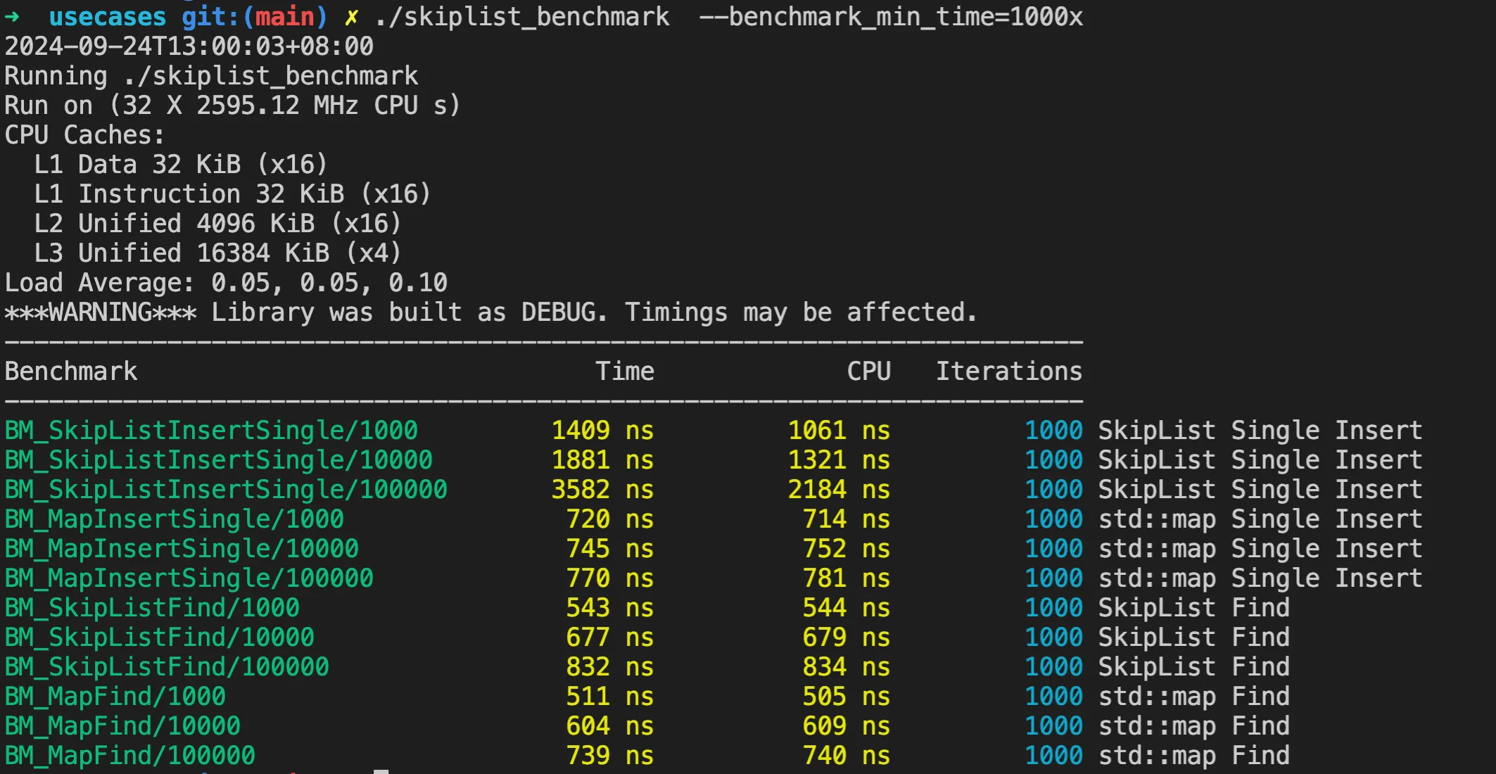
./skiplist_benchmark –benchmark_min_time=1000x
The running results are as follows:

Although this is a Debug version compilation without optimization, we can see from the test results that even as the skip list length increases, the insertion time doesn’t increase significantly. The search performance, compared to unordered_map, isn’t very different either.
Summary
This is the last article on LevelDB skip lists, providing a detailed analysis of the time complexity of skip lists. Through breaking down the search problem, reversing the entire search process, and finding an appropriate L level, we finally derived the time complexity of skip lists. Based on the understanding of time complexity, we further deduced how to choose the probability p, and the reasons for choosing the maximum height in Redis and LevelDB skip lists. Finally, we tested the performance of skip lists through a simple benchmark and compared it with unordered_map.
The other two articles in this series:

